
Task
The task is to use deep learning models to perform weather forecasting over India. This is achieved by predicting meteorological variables, such as temperature and precipitation, based on past data. The task is structured as a regression problem where the model attempts to predict continuous values (e.g., temperature, precipitation amounts).
Dataset
IMDAA Regional Reanalysis Dataset, Available from the IMDAA Reanalysis Portal. Made by India Meteorological Department (IMD), National Centre for Medium Range Weather Forecasting (NCMRWF), Indian Institute of Tropical Meteorology (IITM)
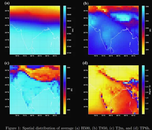
The key variables used for prediction include:
- Geopotential height at 500 hPa (H500),
- Temperature at 850 hPa (T850),
- Temperature at 2m (T2m),
- Six hourly accumulated precipitation (TP6h)
The dataset is divided into three distinct periods for the purpose of training, validation, and testing the model. The training data spans from the year 1990 to 2017, providing a comprehensive dataset for the model to learn from. The year 2018 is designated as the validation period, allowing for the fine-tuning of the model’s parameters and helping to prevent overfitting. Finally, the test data covers the years 2019 to 2020, enabling the assessment of the model’s performance on unseen data.
Loss Metrics
The CNN and LSTM models were evaluated using the following metrics:
- RMSE (Root Mean Squared Error): Measures the standard deviation of the residuals, indicating how much the predictions deviate from the actual values.
- MAE (Mean Absolute Error): Represents the average magnitude of the errors in the predictions.
- ACC (Accuracy): Represents the proportion of correctly predicted values out of the total predictions.
CNN Model
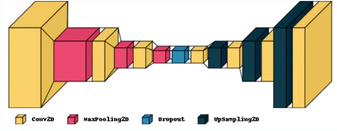
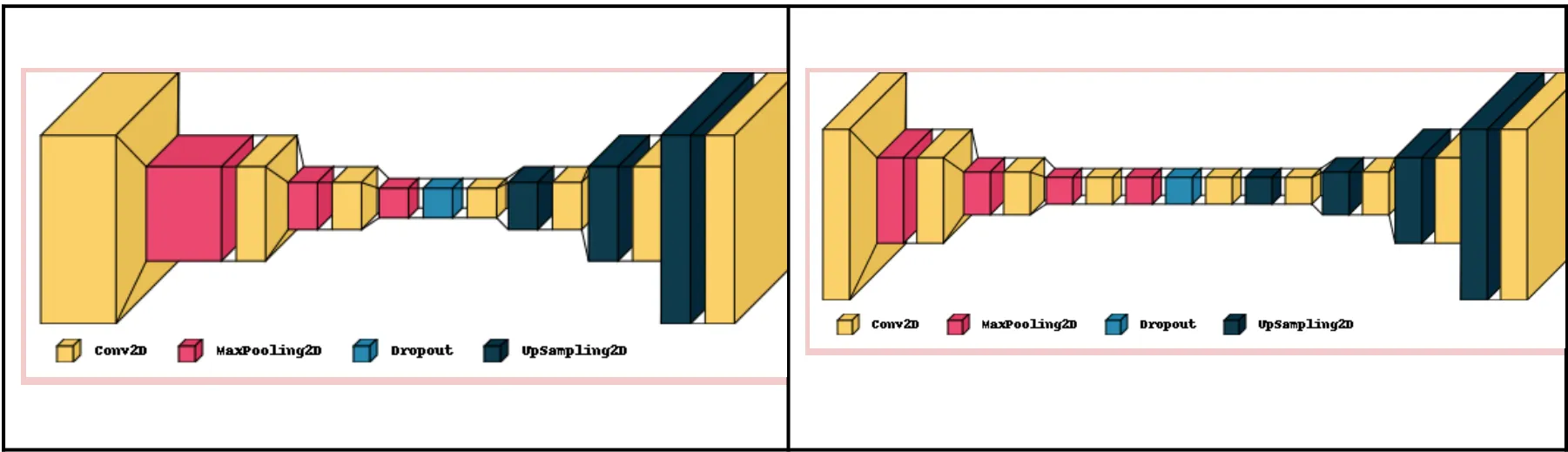
A CNN model was applied to weather data prediction, focusing on the architecture choices that contributed to its performance and stability.
# Build CNN Model
model_cnn = keras.Sequential([
Conv2D(32, 5, padding='same', activation='swish'),
MaxPooling2D(),
Conv2D(32, 5, padding='same', activation='swish'),
MaxPooling2D(),
Conv2D(32, 5, padding='same', activation='swish'),
MaxPooling2D(),
Conv2D(32, 5, padding='same', activation='swish'),
MaxPooling2D(),
Dropout(0.2),
Conv2D(32, 5, padding='same', activation='swish'),
UpSampling2D(),
Conv2D(32, 5, padding='same', activation='swish'),
UpSampling2D(),
Conv2D(32, 5, padding='same', activation='swish'),
UpSampling2D(),
Conv2D(32, 5, padding='same', activation='swish'),
UpSampling2D(),
Conv2D(1, 5, padding='same')
])
# Compile the model
model_cnn.build(X_train[:32].shape)
model_cnn.compile(keras.optimizers.Adam(learning_rate=1e-5), 'mse')
model_cnn.summary()
# Define callbacks
filepath = 'IMDAA_CNN_H500_5days.keras'
checkpoint = ModelCheckpoint(filepath=filepath, monitor='val_loss', verbose=1, save_best_only=True, mode='min')
early_stop = EarlyStopping(monitor="val_loss", patience=5, verbose=1)
# Train the model
def fit_model(model):
history = model.fit(X_train, Y_train, epochs=10,
validation_data=(X_valid, Y_valid),
batch_size=32, shuffle=False,
callbacks=[early_stop, checkpoint])
return history
history_cnn = fit_model(model_cnn)
# Plot training history
plt.plot(history_cnn.history['loss'], label='train')
plt.plot(history_cnn.history['val_loss'], label='test')
plt.xlabel('Epochs')
plt.ylabel('Loss')
plt.legend()
plt.show()
Model Architecture
-
Convolutional Layers
- Multiple convolutional layers were used to extract features from the input data.
- Each layer was followed by:
- Batch Normalization: Helps stabilize training by normalizing inputs.
- Swish Activation Function: Combines input ( x ) with its sigmoid function, improving gradient flow and mitigating vanishing gradients.
- Formula:
Swish(x) = x * σ(x), whereσ(x) = 1 / (1 + exp(-x)). - Cited by Kılıçarslan et al. (2021) as a better alternative to ReLU for many tasks, including image processing.
- Formula:
-
Pooling Layers
- Employed max pooling layers to:
- Reduce spatial dimensions of data.
- Capture essential features without increasing computational load.
- Employed max pooling layers to:
-
Dense Layers
- After flattening convolutional output:
- Dense layers were used to learn the final prediction.
- After flattening convolutional output:
-
Batch Normalization
- Batch Normalization (BatchNorm) was applied throughout to improve the training speed and stability by normalizing layer inputs.
** Performance ** The original CNN model achieved reasonable performance on the evaluation metrics, indicating its effectiveness in predicting the weather data.
Trying some Improvements
Activation Function
The activation function was changed from the Swish function to the Scaled Exponential Linear Unit (SELU) function, defined as follows:
-
selu(x) = λxifx > 0 -
selu(x) = αe^x - αifx ≤ 0 -
λandαare predefined constants; this requires specific weight initialization but is self-normalizing. This helps to:- Keep the mean and variance of inputs to each layer normalized throughout the network.
- Stabilize the training process and ensure faster convergence.
Activation functions introduce non-linearity into the model, which is essential for handling complex data patterns. Without it, a neural network would be equivalent to a linear regression model, regardless of depth.
Removal of Batch Normalization
Batch Normalization can benefit neural networks in several ways:
- It can speed up training by reducing internal covariate shift.
- It acts as a regularizer, potentially reducing the need for Dropout in some cases.
- It can make the model less sensitive to weight initialization.
- It allows for higher learning rates without risking instability, speeding up the training process.
However, using the SELU activation function, which provides self-normalization, reduces the need for Batch Normalization. In practice, removing Batch Normalization was found to yield better results, making its removal an improvement over the original configuration.
ConvLSTM Model
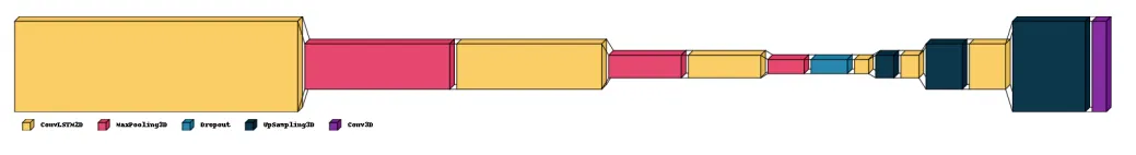
A ConvLSTM (Convolutional Long Short-Term Memory) model, developed to capture spatiotemporal patterns in weather data by integrating convolutional layers with LSTM layers.
ConvLSTM models have been effective in handling sequences of spatial data. For example, Hou et al. (2022) demonstrated that a CNN-LSTM model, separating spatial and temporal components, was an effective predictor of hourly air temperature in China from 2000-2020.
# Reshape the data for ConvLSTM
X_train = X_train[:, np.newaxis, :, :, :]
Y_train = Y_train[:, np.newaxis, :, :, :]
X_valid = X_valid[:, np.newaxis, :, :, :]
Y_valid = Y_valid[:, np.newaxis, :, :, :]
X_test = X_test[:, np.newaxis, :, :, :]
Y_test = Y_test[:, np.newaxis, :, :, :]
# Build ConvLSTM Model
model_conv_lstm = keras.Sequential([
ConvLSTM2D(filters=32, kernel_size=(5, 5), padding="same", return_sequences=True, activation='swish'),
MaxPooling3D(pool_size=(1, 2, 2)),
ConvLSTM2D(filters=32, kernel_size=(5, 5), padding="same", return_sequences=True, activation='swish'),
MaxPooling3D(pool_size=(1, 2, 2)),
Dropout(0.2),
ConvLSTM2D(filters=32, kernel_size=(5, 5), padding="same", return_sequences=True, activation='swish'),
UpSampling3D(size=(1, 2, 2)),
ConvLSTM2D(filters=32, kernel_size=(5, 5), padding="same", return_sequences=True, activation='swish'),
UpSampling3D(size=(1, 2, 2)),
Conv3D(filters=1, kernel_size=(5, 5, 5), padding="same")
])
# Compile the model
model_conv_lstm.build((None, 1, X_train.shape[2], X_train.shape[3], X_train.shape[4]))
model_conv_lstm.compile(keras.optimizers.Adam(learning_rate=1e-6), 'mse')
model_conv_lstm.summary()
# Define callbacks
filepath = 'IMDAA_convlstm_H500_3days.keras'
checkpoint_conv_lstm = ModelCheckpoint(filepath=filepath, monitor='val_loss', verbose=1, save_best_only=True, mode='min')
early_stop_conv_lstm = EarlyStopping(monitor="val_loss", patience=5, verbose=1)
# Train the ConvLSTM model
history_conv_lstm = model_conv_lstm.fit(X_train, Y_train, epochs=5,
validation_data=(X_valid, Y_valid),
batch_size=32, shuffle=False,
callbacks=[early_stop_conv_lstm, checkpoint_conv_lstm])
# Plot training history
plt.plot(history_conv_lstm.history['loss'], label='train')
plt.plot(history_conv_lstm.history['val_loss'], label='test')
plt.xlabel('Epochs')
plt.ylabel('Loss')
plt.legend()
plt.show()
Model Architecture
The ConvLSTM model includes the following components:
- ConvLSTM2D Layers: These layers combine convolutional operations with LSTM units to learn spatiotemporal features from the input data.
- Pooling and UpSampling Layers: Max pooling and upsampling layers manage spatial dimensions and recover the original input size.
- Dropout: Applied to reduce overfitting by randomly setting a fraction of input units to zero during training.
- Batch Normalization: Similar to the CNN model, batch normalization normalizes activations of each layer to maintain zero mean and unit variance.
Performance
The performance of the ConvLSTM model was not satisfactory, showing higher errors compared to the CNN model. This indicates that while ConvLSTM has potential, further tuning or architecture adjustments may be necessary for improved accuracy in weather prediction tasks.
Experiment
Research Question
This experiment is to learn more about the behavior of the original CNN and convLSTM models mentioned in the paper, and with different types of architecture and hyperparameters, to try to improve the loss function and evaluation metrics obtained in the original research to see if a better tuned convLSTM can perform equal to or better than CNN due to its ability of being a spatio temporal model.
Design
Hypothesis: Changes made to hyperparameters and the overall model structure will improve their performance on the given dataset, reducing the error obtained and increasing anomaly correction, and the performance of convLSTM will be equal to or better than CNN at weather prediction.
Independent Variables (Experimental Settings)
- Activation function
- Number of layers
- Number of filters
- Filter size
Control Variables (Biases and Modeling Assumptions)
- Number of epochs will remain constant (10 for CNN, 5 for convLSTM)
- Dataset will stay the same
- Learning rate, optimizer (Adam), and number of batches will remain the same
- Type of pooling will remain MaxPooling
Dependent Variables (Result Analysis)
- Training loss metrics curve over the number of epochs
- Evaluation metrics mentioned above (RMSE, MAE, ACC)
Methodology: The baseline for this experiment is the use of the original BharatBench dataset for weather prediction and the existing implementation on CNN and convLSTM provided by the original authors for comparison. In order to improve the accuracy of the model, initial focus remained on evaluation metrics of RMSE, MAE and ACC, as used by the authors. The following changes were made in order to reach an optimal solution upon continuous adjustments:
CNN Model
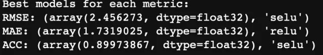
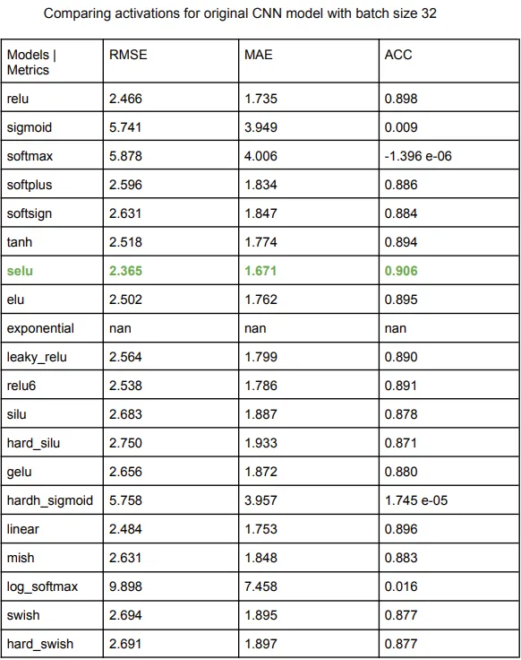
Starting with an analysis of which would be the most optimal activation function for the model (originally ‘swish’), ran 10 epochs for each activation type on the original CNN model and measured the evaluation metrics. Activation ‘selu’ was the best out of all, displayed by an overall metric evaluation.
The original paper mentions batch normalization as a way to improve training of deep neural networks by normalizing input to each layer, which was evaluated in a separate file but not included in the layer architecture due to bad performance metrics. An attempt was also made to change the number of batches to 128 and 64 from 32, which could potentially increase the stability of the optimization, but it also worsened the errors slightly when comparing activations again.
Normally such problems do not need padding changes, so the main focus was on the filters and their dimensions. Increasing the number of filters means more parameters to train on, but risks overfitting the data. Layer manipulation was done by changing the number of layers while tuning the filter size, default stride, as follows:
- Decreased 1 inner layer: Slight Improvement
- Decreased 1 more inner layer and increased filters in layer 2 to 64: Time taken increased to 12 ms/step, Slight Improvement
- Increased number of filters in layer 1 to 512 to recognize more complex patterns: Slight Improvement
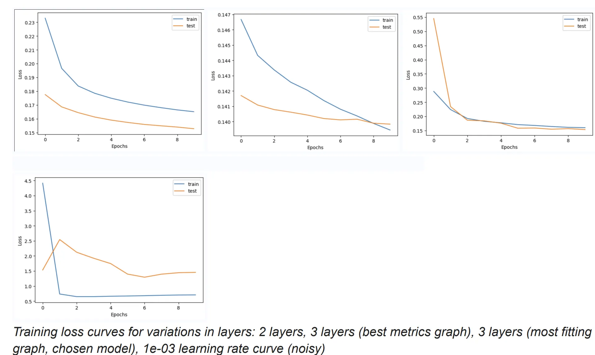
- Increased 1 inner layer [Best Metrics]
- Increased learning rate to 1e-04: Time taken was approximately 17 ms/step [Best Graph] [Chosen Model]
- Same layers, increased learning rate to 1e-03, Big Downgrade
- Same layers, decreased learning rate back to 1e-04 and decreased drop rate from 0.3 to 0.2, Slight Downgrade
No. 4 had the best evaluation metrics results, but upon analysis of their graphs, it was noticed that the graph for No. 5 for loss during training was significantly better, so that was chosen as the optimal model. Modified CNN is also trained for 10 epochs, to compare to original.
ConvLSTM Model
The same activation function was determined to be the best for convLSTM (‘selu’). The model was trained for 1 epoch due its complexity and time elapsed per epoch step being comparatively higher than CNN. Changes to the model architecture and hyperparameters were made as follows:
- Layers with 512,64,64,32 number of filters: Increased time significantly
- Layers with 128,64,64,32 number of filters: Reduced time, reduced accuracy
- Same layers, learning rate increase to 1e-04: Reduced time, increased accuracy
- 1 less layer: Reduced time, increased accuracy
- Layers with 128,128,128 number of filters, drop rate increased to 0.3: 58 ms/step time elapsed, Increased time, Increased accuracy [Chosen Model]
Trying to increase the batches here worsened error and increased the time taken significantly, so it remained 32.
Trying other data variables from the dataset
Original paper noted variable T850 as the best, named TMP_prl. Variables of APCP_sfc and TMP_2m were also tested against both new models. Comparing the models again for the best activation for these new variables, the answer remained ‘selu’.
Results and discussion
CNN model
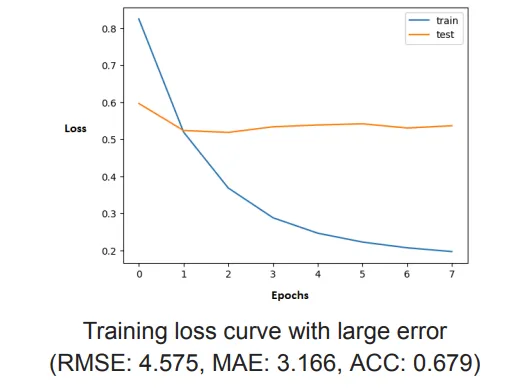
Adding Batch Normalization
Adding Batch Normalization after the Convolution layers resulted in decreased performance of the mode (increased Errors and decreased ACC). Also the loss is very high and increases with increase in epochs.
Possible reasons why Batch Normalization might not have worked:
- Adding batch normalization increases the number of parameters and complexity of the model. For this specific dataset and task, this added complexity might have been unnecessary or even detrimental.
- The nature of weather data, which often involves time series and spatial correlations, might not benefit from the normalization that BatchNorm provides.
- Batch normalization can sometimes lead to overfitting, especially on smaller datasets.
- Batch normalization performance can be sensitive to batch size. If the batch size is too small, the estimates of mean and variance might not be accurate, which can degrade performance.
Batch normalization can allow for higher learning rates. After adding batch normalization, it is suggested to adjust the learning rates which might lead towards optimal performance. This venue can be considered for further experiments to improve the performance of the model.
Changing Activation Functions
The model was tested with various activation functions and it was found that the performance with ‘selu’ (Scaled Exponential Linear Unit) was the best. However, the exponential activation function faced gradient explosion. Increasing the batch size to 64 or 128 in an attempt to increase stability did not improve the gradient explosion issue.
Modifying Layers of the Model
Changing the number of layers by either decreasing or increasing, CNN performs better with 2 layers before and after dropout (not counting pooling), with the best metrics, low errors and high ACC. This suggests that a simpler model architecture with fewer layers is more effective for the specific problem, possibly due to reduced overfitting and more efficient learning of relevant features. However, the learning loss curves obtained by a 3 layer architecture after fine tuning seemed to fit better and converge. These readings were highly sensitive to learning rate changes, so it was challenging to not overfit to the data. The findings indicate that a moderately deeper architecture with an appropriately high learning rate can enhance the model’s ability to learn complex patterns efficiently, striking a balance between underfitting and overfitting. Increasing the number of filters improved the performance of the model slightly. Here are some graphs after the various changes mentioned:
Different layer changes and hyperparameters error metrics
| RMSE | MAE | ACC | |
|---|---|---|---|
| Original CNN | 2.584 | 1.821 | 0.887 |
| Adding Batch Normalization | 4.575 | 3.166 | 0.679 |
| New CNN 4 layers | 2.318 | 1.627 | 0.910 |
| New CNN 3 layers | 2.289 | 1.607 | 0.912 |
| New CNN 2 layers | 2.269 | 1.588 | 0.914 |
| New CNN 2 layers, more filters | 2.248 | 1.576 | 0.915 |
| New CNN 3 layers, same learning rate | 2.220 | 1.553 | 0.918 |
| New CNN 3 layers with more filters in inner layer, higher lr | 2.337 | 1.646 | 0.910 |
| New CNN 3 layers with higher learning rate | 2.334 | 1.685 | 0.910 |
| New CNN 3 layers, higher learning rate, drop rate 0.2 | 2.338 | 1.649 | 0.910 |
The new model for TMP_2m variable from the dataset, vs old model:
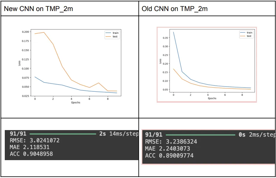
New vs Old CNN:
ConvLSTM Model
Adjsuting Batch Size
Increasing the batch size from 32 to 128 resulted in worsened error metrics and significantly increased the epoch time. Larger batch sizes lead to less frequent updates to the model weights, which can slow convergence and reduce the ability to escape local minima. Smaller batch sizes can add more noise in gradient updates, helping improve generalization and regularization.
Optimizing Learning Rate
Original learning rate was very low at 1e-06, which hindered the training process. Increasing the learning rate to 1e-04 led to substantial performance improvements. A higher learning rate helps the model converge faster by making more significant updates to the weights during training, provided it is not too high to destabilize the training
Experimenting with number of filters
Initially, we configured the model with (512, 64, 64, 32) filters respectively across the four layers in both the encoder and decoder sections. This setup resulted in high runtime due to the large number of parameters. To reduce runtime, we adjusted the filters to (128, 64, 64, 32) respectively. Although this reduced the runtime, it also worsened the model’s performance, likely due to insufficient capacity to capture the complexity of the data.
Reducing model complexity
Removing one layer and using (128, 64, 64) filters in the remaining layers improved performance further. This suggests that the original four-layer configuration might have been overly complex, leading to potential overfitting or inefficient learning
Fine-tuning Filter Configuration and Dropout Rate
Modified the filters to (128, 128, 128) and increased the dropout rate from 0.2 to 0.3. This configuration achieved the best performance with an RMSE: 2.784, MAE: 1.958, ACC: 0.876. The increased dropout rate helped regularize the model, preventing overfitting and improving generalization. Despite the higher training time compared to the original setup, the performance gains justified the trade-off.
Further Increasing Filters
Although increasing the number of filters beyond (128, 128, 128) led to improved performance, it came at the cost of significantly higher training time. This trade-off between performance and training time needs careful consideration depending on the application’s requirements.
Observations
The experiments with the ConvLSTM model revealed that balancing the number of filters, batch size, and learning rate is crucial for optimizing performance. While higher filter counts and learning rates can improve accuracy and reduce errors, they also increase training time. Similarly, smaller batch sizes can help the model generalize better but may slow down training.
The best-performing model configuration was achieved with (128, 128, 128) filters, a dropout rate of 0.3, and a learning rate of 1e-04, providing a good balance between performance and training efficiency.
This optimal configuration was then applied to two other variables in the dataset. However, the model performed poorly on these variables, indicating that the configuration tuned for tmp_prl did not generalize well to other variables (tmp_2m and aspc). This emphasizes the need for individualized tuning to address the distinct characteristics of each variable. Each variable in the dataset may have unique characteristics and patterns that require tailored model configurations. Factors such as data distribution, underlying trends, and the complexity of temporal patterns can vary significantly between variables, impacting the model’s ability to perform well in a general manner.
The evaluation metrics are not the sole indicator of which algorithm is better. Even though the training loss curve and the error metrics were better for our new model on dataset variable TMP_prl (the one finally used in the paper), evaluation on another metric TMP_2m gave a drastically different looking loss curve even though the error is still less in comparison. Moreover, APCP_sfc was giving very bad results and is excluded from this comparison. Although we were finally able to improve the overall performance of the model, the model needs to be tuned independently for all the variables of the dataset in order to perform better as they all might have different characteristics.
ConvLSTM’s performance did not change much for this new dataset variable, so using the original variable as intended here as well. Hence, the hypothesis that ConvLSTM would show comparable performance to CNN has failed.
Future
- (Not completed) Making a Spherical CNN to take into account the 3D nature of weather physics, and trying to include numerical methods of fluid dynamics into the model for better predictions.
# Install s2cnn library for spherical convolutions
!pip install s2cnn
import torch
import torch.nn as nn
from s2cnn import S2Convolution, SO3Convolution
# Define the spherical CNN model
class SphericalCNN(nn.Module):
def __init__(self):
super(SphericalCNN, self).__init__()
# Spherical convolutional layers
self.s2conv1 = S2Convolution(nfeature_in=1, nfeature_out=32, b_in=30, b_out=20)
self.s2conv2 = S2Convolution(nfeature_in=32, nfeature_out=64, b_in=20, b_out=10)
self.s2conv3 = S2Convolution(nfeature_in=64, nfeature_out=128, b_in=10, b_out=5)
self.s2conv4 = S2Convolution(nfeature_in=128, nfeature_out=256, b_in=5, b_out=3)
# Fully connected layers
self.fc1 = nn.Linear(256 * 3 * 3, 64)
self.fc2 = nn.Linear(64, 1)
# Pooling and dropout layers
self.pool = nn.MaxPool1d(kernel_size=2, stride=2)
self.dropout = nn.Dropout(p=0.3)
def forward(self, x):
# Pass through spherical convolutions, activation, and pooling
x = self.pool(nn.functional.relu(self.s2conv1(x)))
x = self.pool(nn.functional.relu(self.s2conv2(x)))
x = self.pool(nn.functional.relu(self.s2conv3(x)))
x = self.pool(nn.functional.relu(self.s2conv4(x)))
# Flatten and pass through fully connected layers
x = x.view(x.size(0), -1)
x = nn.functional.relu(self.fc1(x))
x = self.dropout(x)
x = self.fc2(x)
return x
# Instantiate model, define loss and optimizer
model = SphericalCNN()
criterion = nn.MSELoss()
optimizer = torch.optim.Adam(model.parameters(), lr=1e-4)
print(model)
Refernces
- Choudhury, A., Panda, J., & Mukherjee, A. (2024). BharatBench: Dataset for data-driven weather forecasting over India. arXiv [Physics.Ao-Ph]. arXiv: 2405.07534
- Michel Jose Anzanello, Flavio Sanson Fogliatto,Learning curve models and applications: International Journal of Industrial Ergonomics, Volume 41, Issue 5, 2011, Pages 573-583, ISSN 0169-8141,DOI: 10.1016/j.ergon.2011.05.001
- Kılıçarslan, S., Adem, K., & Çelik, M. (2021). An overview of the activation functions used in deep learning algorithms. Journal of New Results in Science, 10(3), 75-88. DOI: 10.54187/jnrs.1011739
- Hou, J., Wang, Y., Zhou, J., & Tian, Q. (2022). Prediction of hourly air temperature based on CNN–LSTM. Geomatics, Natural Hazards and Risk,13(1), 1962–1986. DOI: 10.1080/19475705.2022.2102942