List of Symbols

NAME	SYMBOL
Chord length of hydrofoil, m	c
Reynold’s number based on chord length	Re
Area of hydrofoil, m²	A
Lift coefficient	c_l
Drag coefficient	c_d
Pressure coefficient	c_p
Reynold’s averaged velocity, m/s	u_i
Freestream velocity, m/s	U_∞
Local static pressure, Pa	p
Vapor pressure of liquid, Pa	p_v
Freestream pressure, Pa	p_∞
Evaporation rate, kg/(m³ s)	R_e
Condensation rate, kg/(m³ s)	R_c
Angle of attack, °	α
Cavitation number	σ
Molecular viscosity, Pa s	μ
Viscosity of water, Pa s	μ_l
Viscosity of water-vapor, Pa s	ν_v
Turbulent viscosity, Pa s	μ_t
Effective viscosity, Pa s	μ_eff
Turbulent kinetic energy, m²/s²	K
Rate of dissipation of turbulent kinetic energy, m²/s³	E
Vapor volume fraction	α_v
Liquid density, kg/m³	ρ_l
Vapor density, kg/m³	ρ_v
Mixture density, kg/m³	ρ_m

Equations

The most common model used to solve the cavitating flow is the homogeneous mixture model. In this model, the pressure, temperature, and velocity between the phases are equal. The governing equations for this mixture model involve solving the unsteady Reynold’s Navier–Stokes (URANS) equations using the turbulence model.

\frac{\partial \rho_m}{\partial t} + \frac{\partial (u_j \rho_m)}{\partial x_j} = 0,\tag{1}

\frac{\partial (\rho_m u_i)}{\partial t} + \frac{\partial (\rho_m u_i u_j)}{\partial x_j} = -\frac{\partial p}{\partial x_i} + \frac{\partial}{\partial x_j} \left[ \mu_{eff} \left( \frac{\partial u_i}{\partial x_j} + \frac{\partial u_j}{\partial x_i} - \frac{2}{3} \frac{\partial u_k}{\partial x_k} \right) \right]\tag{2}

\rho_m \text{ - fluid mixture density}

u_i \text{ - Reynold's averaged velocity}

p \text{ - local static pressure}

\mu_{eff} \text{ - effective viscosity, the sum of molecular viscosity and turbulent viscosity}

Effective Viscosity

\mu_{eff} = \mu + \mu_t \tag{3}

For K-E turbulence model

\mu_t = \rho_m C_\mu \frac{K^2}{E} \tag{4}

K \text{ - turbulent kinetic energy}

E \text{ - rate of dissipation of kinetic energy}

C_μ is the model parameter. The Realizable K−E model does not assume C_μ as a constant. Instead, C_μ varies according to the flow field to satisfy the physics of turbulent flows (Reynolds, 1987).

\text{The fluid mixture density } \rho_m \text{ using the Zwart–Gerber–Belamri cavitation model.}

\rho_m = \alpha_v \rho_v + (1 - \alpha_v) \rho_l \tag{5}

\alpha_v \text{ - vapor volume fraction}

\rho_v \text{ - vapor density}

\rho_l \text{ - liquid density}

Turbulence model

In cavitating flows, the Realizable κ − model found to be more effective than other models (Shih et al. 1995). The modelled transport equations for turbulent kinetic energy (K) and its rate of dissipation (E ) for Realizable K − E model are (Shih et al. 1995)

\frac{\partial (\rho_m K)}{\partial t} + \frac{\partial (\rho_m K u_i)}{\partial x_j} = \frac{\partial}{\partial x_j} \left( \mu + \frac{\mu_t}{\sigma_K} \frac{\partial K}{\partial x_j} \right) + G_K - \rho_m - Y_M \tag{6}

\frac{\partial (\rho_m E)}{\partial t} + \frac{\partial (\rho_m E u_i)}{\partial x_j} = \frac{\partial}{\partial x_j} \left( \mu + \frac{\mu_t}{\sigma_E} \frac{\partial E}{\partial x_j} \right) - \rho_m C_2 \frac{E^2}{K + \sqrt{\nu E}} \tag{7}

G_K \text{ - Turbulent Kinetic Energy due to mean velocity gradients}

Y_M \text{ - Contribution of the fluctuating dilatation in compressible turbulence}

\text{to the overall dissipation rate.}

C_2 = 1.9, \, \sigma_K = 1.0, \, \sigma_E = 1.2 \text{ are model constants}

Cavitation Model

Zwart–Gerber–Belamri cavitation model is used to determine the vapor volume fraction. The transport equation for this model is given as (Nied´zwiedzka 2017)

\frac{\partial (\rho_v \alpha_v)}{\partial t} + \frac{\partial (u_j \alpha_v \rho_v)}{\partial x_j} = R_e - R_c \tag{8}

R_e \text{ and } R_c \text{ are source terms related to evaporation and condensation of vapor bubbles.}

R_e = F_{vap} \frac{3 \alpha_{nuc} (1 - \alpha_v) \rho_v}{R_b} \sqrt{\frac{2}{3}} \sqrt{\frac{(p - p_{sat})}{\rho_l}} \tag{9}

R_c = - F_{cond} \frac{3 \alpha_v \rho_v}{R_b} \sqrt{\frac{2}{3}} \sqrt{\frac{(p_{sat} - p)}{\rho_l}} \tag{10}

R_b \text{ - Radius of the bubble, } R_b = 10^{-6} \, \text{m}

p_{sat} \text{ - Saturation pressure of the liquid}

\text{ Evaporation Coefficient, } F_{vap} = 50

\text{ Condensation Coefficient, } F_{cond} = 0.001

\text{ Nucleation site Volume Fraction, } \alpha_{nuc} = 0.0005

Performance Parameters

Cavitation number (σ), pressure coefficient (C_p), lift coefficient (C_l), and drag coefficient (C_d) define the hydrodynamic performance of a hydrofoil. The cavitation number (σ) is a nondimensional number that determines the cavity formation on the hydrofoil. It is expressed as the ratio of the difference between local absolute pressure and fluid vapor pressure to dynamic pressure (Brennen 2014).

\sigma = \frac{p - p_v}{\frac{1}{2} \rho U_{\infty}^2} \tag{11}

The pressure coefficient (C_p) is defined as the ratio of the pressure difference on the hydrofoil to the dynamic pressure.

C_p = \frac{p - p_\infty}{\frac{1}{2} \rho U_\infty^2} \tag{12}

The lift coefficient (C_l) represents the nondimensional form of the lift force. Similarly, the drag coefficient (C_d) quantifies the resistive force developed in the opposite direction of fluid flow.

C_l = \frac{Lift}{\frac{1}{2} \rho U_{\infty}^2} \tag{13}

C_d = \frac{Drag}{\frac{1}{2} \rho U_{\infty}^2} \tag{14}

\begin{align*} &U_{\infty} \text{ - Free-stream velocity (m/s)} \\ &\rho \text{ - Density of water (kg/m}^3\text{)} \\ &p_{\infty} \text{ - Pressure at free stream (Pa)} \\ &p_v \text{ - Vapor pressure (Pa)} \end{align*}

Computational Domain

A NACA4418 hydrofoil having 0.1m chord length (c) is simulated using rectangular computational fluid domain. The fluid domain around the hydrofoil is considered to be rectangular with a C type inlet which gives the advantage of reduced computational cost. (Berntsen et al. 2001; Ghadimi et al. 2018; Mokhtar and Zheng 2006; Huang et al. 2010; Karim and Ahmmed 2012). The simulation domain was designed with dimensions of 25.5 times the chord length in the x-direction and 15 times the chord length in the y-direction, to minimize the influence of wall boundary conditions on the flow near the hydrofoil. An inlet with a circular cross-section and a radius of 7.5 times the chord length was positioned at 13.5 times the chord length upstream from the leading edge of the hydrofoil, while the outlet was placed at 12 times the chord length downstream from the leading edge of the hydrofoil.

Number of Cells = 100580

Maximum Aspect Ratio = 4.22647e+02

Minimum Orthogonal Quality = 2.29297e-01

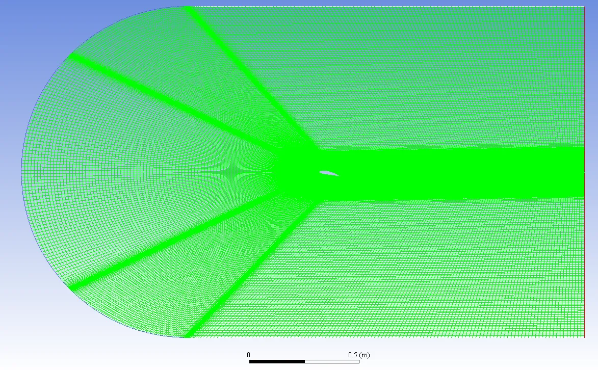Domain Figure 1 : Computational Domain

Boundary conditions

A uniform x-component velocity of 7 m/s is specified at the inlet. Based on the chord length and inlet velocity, the Reynold’s number is 0.7 × 10⁶. The upper and lower walls of the domain are stationary walls set to no slip conditions. All the reference values are mentioned in Table 1.

The Zwart–Gerber–Belamri cavitation model is used to model cavitation. The Realizable K-E turbulence model with enhanced wall treatment is used for the viscosity in the fluid domain. For pressure and velocity coupling, the Coupled scheme is used. This scheme provides robust solutions by solving the pressure and momentum-based continuity equations together (Srijna 2021). For pressure the PRESTO scheme is used and for momentum, volume fraction, turbulent kinetic energy and dissipation rate, the QUICK scheme is used.

Variable	Value
U_∞	7 m/s
ρ_l	998.2 kg/m³
ρ_v	0.55 kg/m³
μ_l	1 × 10^-3
μ_v	1.35 × 10^-5
p_v	3540 Pa
Re	0.7 × 10⁶
c	0.1 m

Results

The results are validated by comparing the pressure coefficients from the simulation to the experimental data of NACA 4418(airfoiltools.com) at high Reynold’s numbers as shown in Fig . The simulation generated pressure coefficients are consistent with experimental data. The hydrofoil’s pressure coefficients at the pressure and suction sides are also compared with the results from Srijna 2021 paper, the angle of attack is the same (12 degrees), but the cavitation numbers are different. The graphs are inverted because negative pressure coefficient is considered in the Srijna 2021 paper. The graphs are for different cavitation numbers, so they are not equal, but they seem to be consistent with each other. The Volume Fraction contours also seem to be consistent with the Srijna 2021 paper.

Pressure and Velocity Distributions

The x-velocity distribution in the domain is displayed in figure 8. The velocity behind the hydrofoil with respect to the fluid flow goes below zero and then to 0, indicating a change in flow direction. This can be explained with the angle of attack and orientation of the hydrofoil, which blocks the incoming flow and creates a low-pressure region. This affects the x-velocity behind the hydrofoil.

X-Velocity σ = 2.3 and α = 12

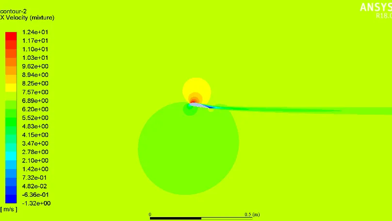
Figure 2 : X-Velocity σ = 2.3 and α = 12

X-Velocity σ = 0.28 and α = 12

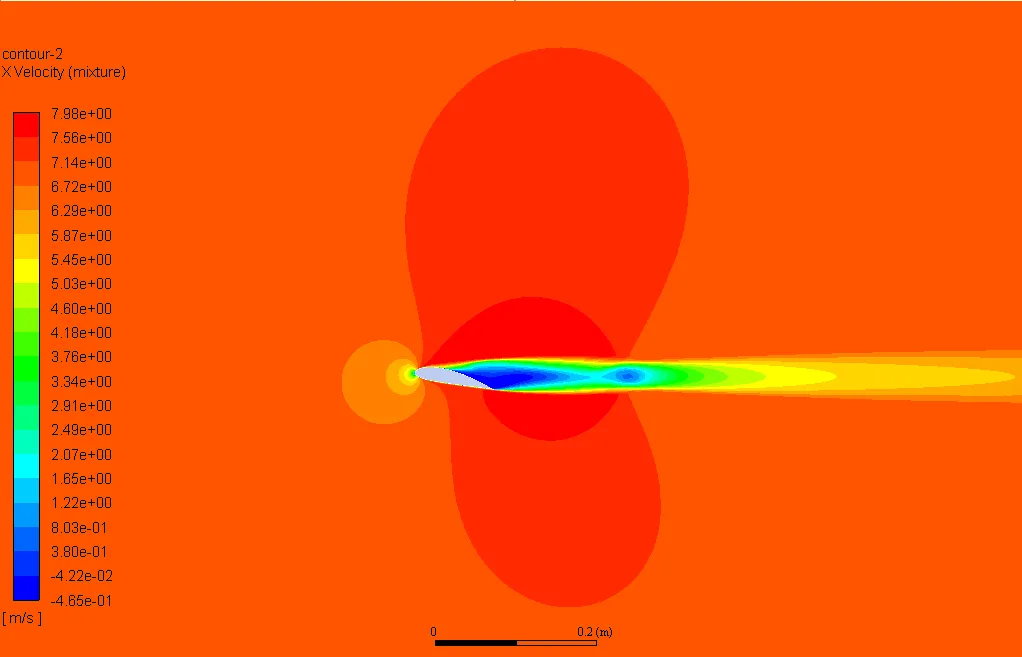
Figure 3 : X-Velocity σ = 0.28 and α = 12

The difference in Cp in the regions above and below the hydrofoil is what enables the lift of the hydrofoil. Due to the presence of the hydrofoil, the entire domain is split into two parts of different pressure coefficients seen in figure 10 & 11. The pressure differences near the hydrofoil are greater than the rest of the domain.

Pressure Coefficient σ = 2.3 and α = 12

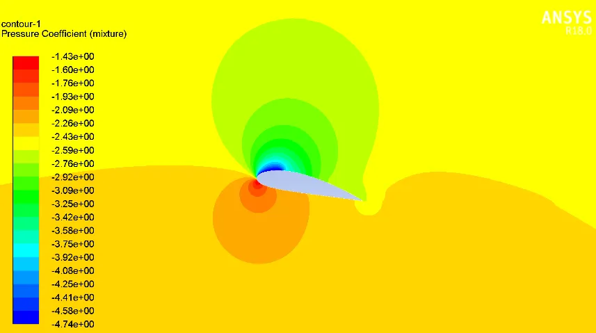
Figure 4 : X-Velocity σ = 2.3 and α = 12

Pressure Coefficient σ = 0.28 and α = 12

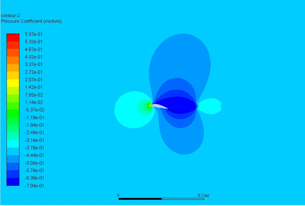
Figure 5 : X-Velocity σ = 0.28 and α = 12

Performance Parameters of the Hydrofoil

The red color indicates the pressure at the upper side (suction side) and the green indicates the pressure at the lower side (pressure side). The 0 m position coincides with the tip of the hydrofoil (Figure 5 & 6). The pressure differences close to the tip of the hydrofoil vary a lot, indicating the lift force is mostly experienced from the tip of the hydrofoil.

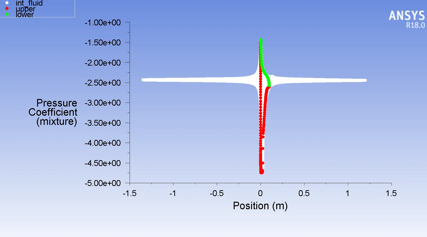
Pressure Coefficient vs X-Position σ = 2.3 and α = 12

Figure 6 : Pressure Coefficient vs X-Position σ = 2.3 and α = 12

Pressure Coefficient vs X-Position σ = 0.28 and α = 12

Figure 7 : Pressure Coefficient vs X-Position σ = 0.28 and α = 12

For σ = 2.3 , The cavity length is determined by considering the x-distance for which the pressure coefficient value on the suction side is below -3 (Zhang 2021). The cavity length is around 0.05m for σ = 2.3 and α = 12. (Figure 7)

For σ = 0.28, The cavity extends beyond the suction side of the hydrofoil and into the fluid domain. In this case, the cavity length is determined by the x-distance for which the pressure coefficient goes below -0.45. The cavity length is around 0.26m for σ = 0.28 and α = 12 (Figure 8). The Volume Fraction contours are given in Figure 10 and 11 for visualization.

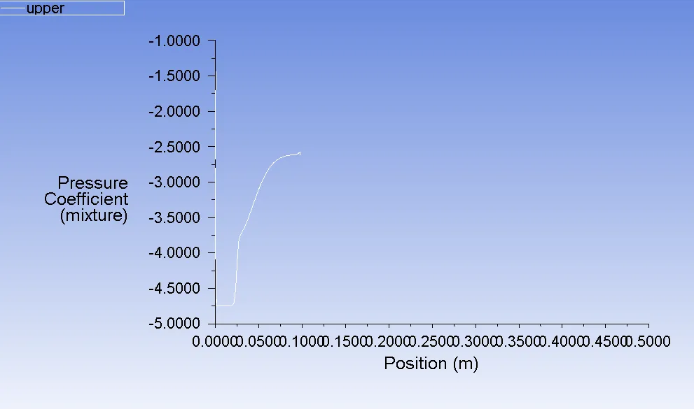
Pressure Coefficient on the suction side vs X-position for σ = 2.3 and α = 12

Figure 8 : Pressure Coefficient on the suction side vs X-position for σ = 2.3 and α = 12

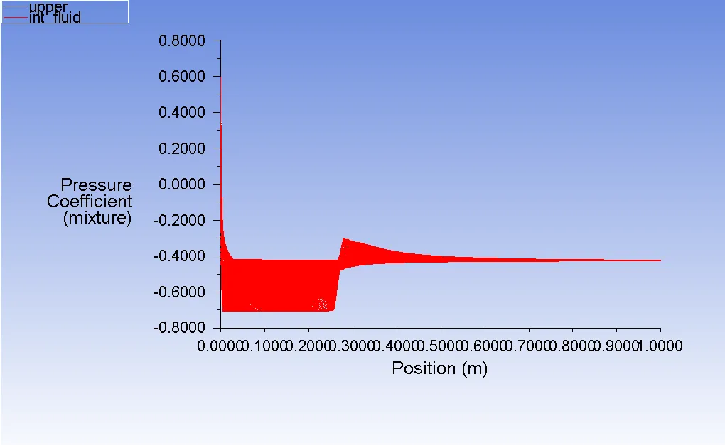
Pressure Coefficient on the suction side vs X-position for σ = 0.28 and α = 12

Figure 9 : Pressure Coefficient on the suction side vs X-position for σ = 0.28 and α = 12

Volume Fraction for σ = 2.3 and α = 12

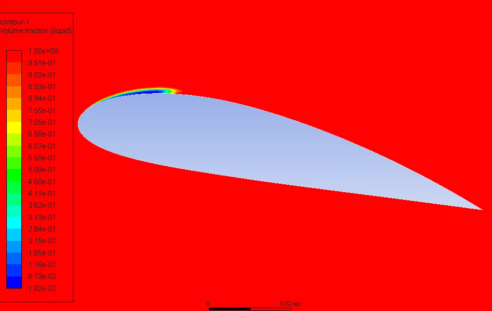
Figure 10 : Volume Fraction for σ = 2.3 and α = 12

Volume Fraction for σ = 0.28 and α = 12

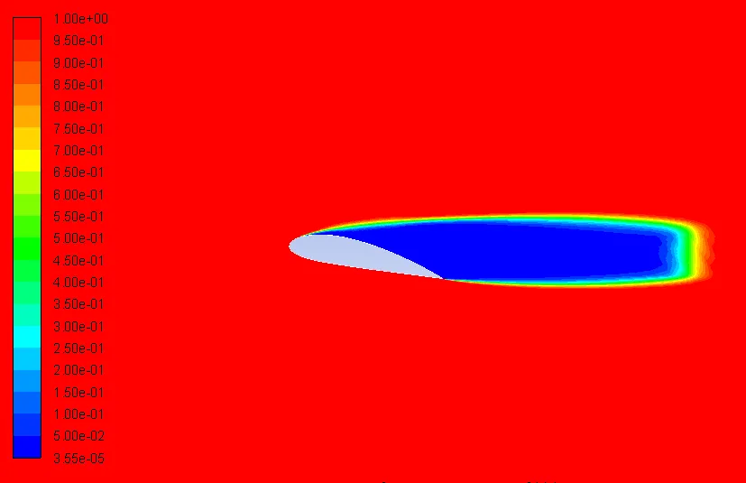
Figure 11 : Volume Fraction for σ = 0.28 and α = 12

The coefficients of lift (C_l) and drag (C_d) are two important aerodynamic coefficients that describe the performance of an airfoil or hydrofoil. The coefficient of lift and drag on the hydrofoil are given in Figure 12, 13, 14, and 15. The cavity length for σ = 2.3 and α = 12 is 0.05 m and the cavity length for σ = 0.28 and α = 12 is 0.26 m.

Cd for σ = 2.3 and α = 12

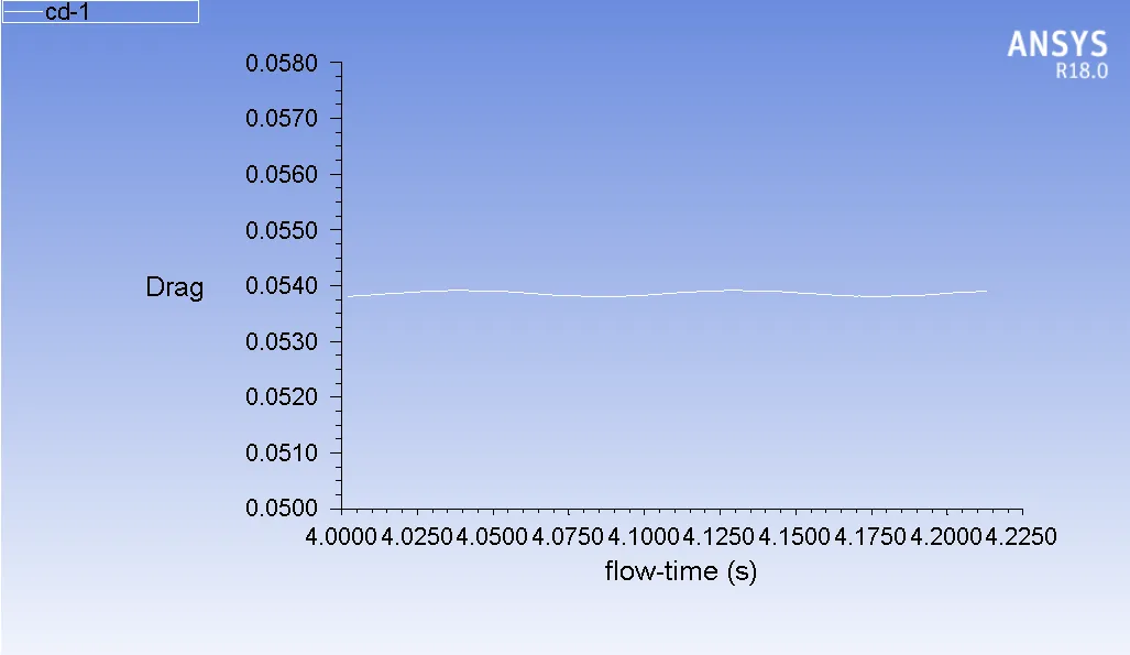
Figure 12 : Cd for σ = 2.3 and α = 12

Cl for σ = 2.3 and α = 12

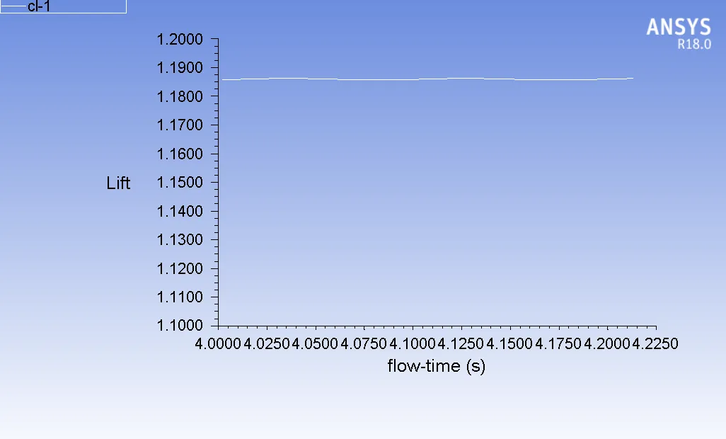
Figure 13 : Cl for σ = 2.3 and α = 12

Cd for σ = 0.28 and α = 12

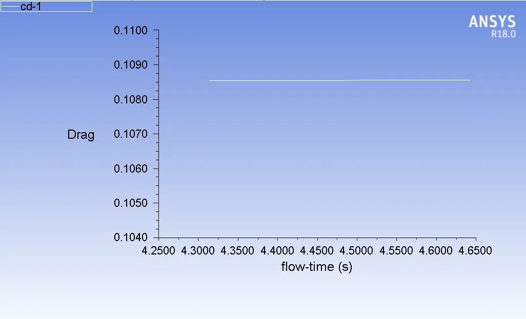
Figure 14 : Cd for σ = 0.28 and α = 12

Cl for σ = 0.28 and α = 12

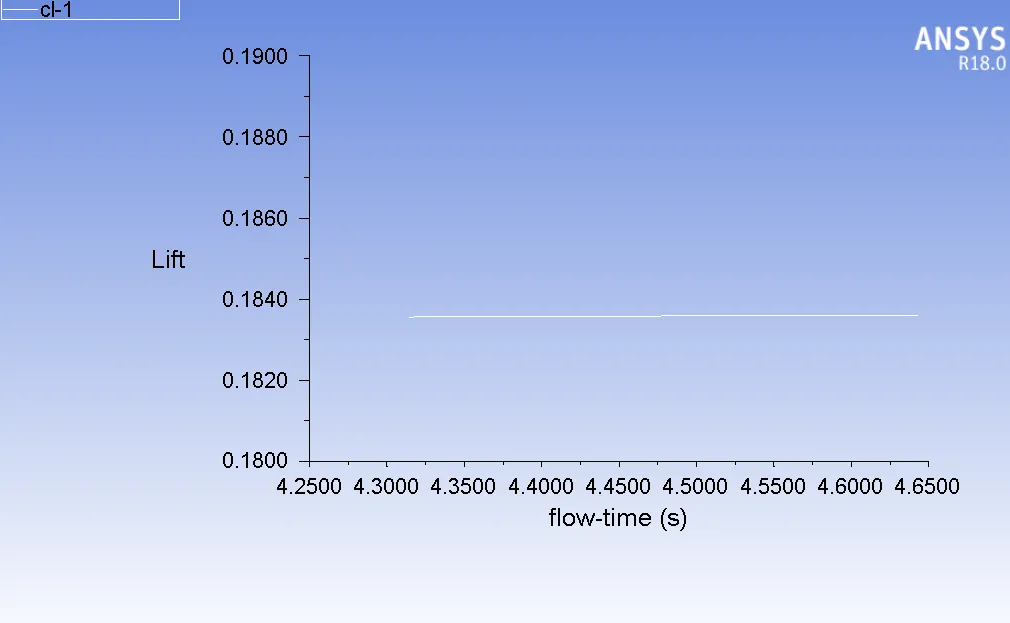
Figure 15 : Cl for σ = 0.28 and α = 12

Performance Parameters Table σ = 0.28 and 2.3

Cavitation Number	2.3	0.28
Lift Coefficient	1.1850	0.1838
Drag Coefficient	0.0538	0.1085
Cavity Length	0.05 m	0.26 m
Maximum Pressure Coefficient	-1.4	0.6
Minimum Pressure Coefficient	-4.7	-0.7

Fluent CFD simulation of converging diverging (CD) nozzle